kmeans | God, Your Book Is Great !!

Posts Tagged ‘kmeans’

Code Snippet to run kMeans clustering in BioPython

Posted in Data Mining, Python, tagged biopython, kmeans on November 21, 2010| 4 Comments »

I recently had to implement kMeans algorithm for clustering genes based on their profiles for one of my bioinformatics homework. Even though, I implemented my code, I wanted to compare the results using BioPython. For those, who do not know, BioPython is a set of libraries that allow you to write bioinformatics code. They have implemented most of the fundamental algorithms in bioinformatics. To me it was a great lifesaver as I can test out my ideas in few lines of Python code.

In Ubuntu, if you want to install it use the command : sudo apt-get install python-biopython .

Anyway, I was searching in net to get a code snippet to do kMeans using BioPython and somehow did not find any. So I wrote one myself using the documentation. I thought I will post code in the blog so that if anyone needs it in the future its a google search away 🙂

Biopython’s kMeans code requires the input to be in the format accepted by Eisner’s treeview program so that needed some data massaging. The code per se is very simple. It provides the data file, number of clusters and the number of runs to try as input. Additionally it also passes an array to initialize the cluster centroids.

from Bio import Cluster
f = open("gData1.csv")
record = Cluster.Record(f)
initialId = []
numClusters = 4
numRecords = 12
for i in range(numClusters):
     for j in range(numRecords/numClusters):
        initialId.append(i)
        #(clusterAssignment, totalError, numPasses) = record.kcluster(nclusters=numClusters,initialid=initialId)
        (clusterAssignment, totalError, numPasses) = record.kcluster(nclusters=numClusters,npass=10)
geneNames = record.genename
g = [ [] for i in range(numClusters)]
numIndex = 0
for i in clusterAssignment :  
     g[i].append(geneNames[numIndex])
     numIndex += 1
f.close()

The input file looks like this : It is a tab separated file with the first two special fields : geneid and gene name.

GENEID  NAME    PARAM1      PARAM2      
BLAH1    BLAH2   -0.43          0.3

Hope the snippet is useful to some !

Read Full Post »

Introduction To Mean Shift Algorithm

Posted in Data Mining, machine learning, tagged clustering, computer vision, convergence, kmeans, matlab, mean shift on April 1, 2010| 88 Comments »

Its been quite some time since I wrote a Data Mining post . Today, I intend to post on Mean Shift – a really cool but not very well known algorithm. The basic idea is quite simple but the results are amazing. It was invented long back in 1975 but was not widely used till two papers applied the algorithm to Computer Vision.

I learned this algorithm in my Advanced Data Mining course and I wrote the lecture notes on it. So here I am trying to convert my lecture notes to a post. I have tried to simplify it – but this post is quite involved than the other posts.

It is quite sad that there exists no good post on such a good algorithm. While writing my lecture notes, I struggled a lot for good resources 🙂 . The 3 “classic" papers on Mean Shift are quite hard to understand. Most of the other resources are usually from Computer Vision courses where Mean Shift is taught lightly as yet another technique for vision tasks (like segmentation) and contains only the main intuition and the formulas.

As a disclaimer, there might be errors in my exposition – so if you find anything wrong please let me know and I will fix it. You can always check out the reference for more details. I have not included any graphics in it but you can check the ppt given in the references for an animation of Mean Shift.

Introduction

Mean Shift is a powerful and versatile non parametric iterative algorithm that can be used for lot of purposes like finding modes, clustering etc. Mean Shift was introduced in Fukunaga and Hostetler [1] and has been extended to be applicable in other fields like Computer Vision.This document will provide a discussion of Mean Shift , prove its convergence and slightly discuss its important applications.

Intuitive Idea of Mean Shift

This section provides an intuitive idea of Mean shift and the later sections will expand the idea. Mean shift considers feature space as a empirical probability density function. If the input is a set of points then Mean shift considers them as sampled from the underlying probability density function. If dense regions (or clusters) are present in the feature space , then they correspond to the mode (or local maxima) of the probability density function. We can also identify clusters associated with the given mode using Mean Shift.

For each data point, Mean shift associates it with the nearby peak of the dataset’s probability density function. For each data point, Mean shift defines a window around it and computes the mean of the data point . Then it shifts the center of the window to the mean and repeats the algorithm till it converges. After each iteration, we can consider that the window shifts to a more denser region of the dataset.

At the high level, we can specify Mean Shift as follows :
1. Fix a window around each data point.
2. Compute the mean of data within the window.
3. Shift the window to the mean and repeat till convergence.

Preliminaries

Kernels :

A kernel is a function that satisfies the following requirements :

1. $\int_{R^{d}}\phi(x)=1$

2. $\phi(x)\geq0$

Some examples of kernels include :

1. Rectangular $\phi(x)=\begin{cases} 1 & a\leq x\leq b\\ 0 & else\end{cases}$

2. Gaussian $\phi(x)=e^{-\frac{x^{2}}{2\sigma^{2}}}$

3. Epanechnikov $\phi(x)=\begin{cases} \frac{3}{4}(1-x^{2}) & if\;|x|\leq1\\ 0 & else\end{cases}$

Kernel Density Estimation

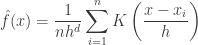
Kernel density estimation is a non parametric way to estimate the density function of a random variable. This is usually called as the Parzen window technique. Given a kernel K, bandwidth parameter h , Kernel density estimator for a given set of d-dimensional points is

$\hat{f}(x)=\frac{1}{nh^{d}}\sum_{i=1}^{n}K\left(\frac{x-x_{i}}{h}\right)$

Gradient Ascent Nature of Mean Shift

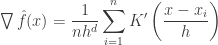
Mean shift can be considered to based on Gradient ascent on the density contour. The generic formula for gradient ascent is ,

$x_{1}=x_{0}+\eta f'(x_{0})$

Applying it to kernel density estimator,

$\hat{f}(x)=\frac{1}{nh^{d}}\sum_{i=1}^{n}K\left(\frac{x-x_{i}}{h}\right)$

$\bigtriangledown{\displaystyle \hat{f}(x)=\frac{1}{nh^{d}}\sum_{i=1}^{n}K'\left(\frac{x-x_{i}}{h}\right)}$

Setting it to 0 we get,

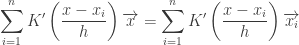
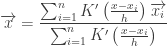
$\sum_{i=1}^{n}K'\left(\frac{x-x_{i}}{h}\right)\overrightarrow{x}=\sum_{i=1}^{n}K'\left(\frac{x-x_{i}}{h}\right)\overrightarrow{x_{i}}$

Finally , we get

$\overrightarrow{x}=\frac{\sum_{i=1}^{n}K'\left(\frac{x-x_{i}}{h}\right)\overrightarrow{x_{i}}}{\sum_{i=1}^{n}K'\left(\frac{x-x_{i}}{h}\right)}$

Mean Shift

As explained above, Mean shift treats the points the feature space as an probability density function . Dense regions in feature space corresponds to local maxima or modes. So for each data point, we perform gradient ascent on the local estimated density until convergence. The stationary points obtained via gradient ascent represent the modes of the density function. All points associated with the same stationary point belong to the same cluster.

Assuming 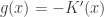$g(x)=-K'(x)$ , we have

$m(x)=\frac{\sum_{i=1}^{n}g\left(\frac{x-x_{i}}{h}\right)x_{i}}{\sum_{i=1}^{n}g\left(\frac{x-x_{i}}{h}\right)}-x$

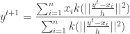
The quantity $m(x)$ is called as the mean shift. So mean shift procedure can be summarized as : For each point $x_{i}$

1. Compute mean shift vector $m(x_{i}^{t})$

2. Move the density estimation window by $m(x_{i}^{t})$

3. Repeat till convergence

Using a Gaussian kernel as an example,

1. $y_{i}^{0}=x_{i}$
2. $y_{i}^{t+1}=\frac{\sum_{i=1}^{n}x_{j}e^{\frac{-|y_{i}^{t}-x_{j}|^{2}}{h^{2}}}}{\sum_{i=1}^{n}e^{\frac{-|y_{i}^{t}-x_{j}|^{2}}{h^{2}}}}$

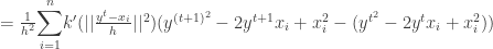
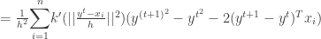
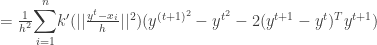
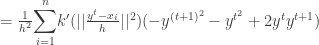
Proof Of Convergence

Using the kernel profile,

$y^{t+1}=\frac{\sum_{i=1}^{n}x_{i}k(||\frac{y^{t}-x_{i}}{h}||^{2})}{\sum_{i=1}^{n}k(||\frac{y^{t}-x_{i}}{h}||^{2})}$

To prove the convergence , we have to prove that 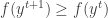$f(y^{t+1})\geq f(y^{t})$

$f(y^{t+1})-f(y^{t})={\displaystyle \sum_{i=1}^{n}}k(||\frac{y^{t+1}-x_{i}}{h}||^{2})-{\displaystyle \sum_{i=1}^{n}}k(||\frac{y^{t}-x_{i}}{h}||^{2})$

But since the kernel is a convex function we have ,

$k(y^{t+1})-k(y^{t})\geq k'(y^{t})(y^{t+1}-y^{t})$

Using it ,

$f(y^{t+1})-f(y^{t})\geq{\displaystyle \sum_{i=1}^{n}}k'(||\frac{y^{t}-x_{i}}{h}||^{2})(||\frac{y^{t+1}-x_{i}}{h}||^{2}-||\frac{y^{t}-x_{i}}{h}||^{2})$

$=\frac{1}{h^{2}}{\displaystyle \sum_{i=1}^{n}}k'(||\frac{y^{t}-x_{i}}{h}||^{2})(y^{(t+1)^{2}}-2y^{t+1}x_{i}+x_{i}^{2}-(y^{t^{2}}-2y^{t}x_{i}+x_{i}^{2}))$

$=\frac{1}{h^{2}}{\displaystyle \sum_{i=1}^{n}}k'(||\frac{y^{t}-x_{i}}{h}||^{2})(y^{(t+1)^{2}}-y^{t^{2}}-2(y^{t+1}-y^{t})^{T}x_{i})$

$=\frac{1}{h^{2}}{\displaystyle \sum_{i=1}^{n}}k'(||\frac{y^{t}-x_{i}}{h}||^{2})(y^{(t+1)^{2}}-y^{t^{2}}-2(y^{t+1}-y^{t})^{T}y^{t+1})$

$=\frac{1}{h^{2}}{\displaystyle \sum_{i=1}^{n}}k'(||\frac{y^{t}-x_{i}}{h}||^{2})(y^{(t+1)^{2}}-y^{t^{2}}-2(y^{(t+1)^{2}}-y^{t}y^{t+1}))$

$=\frac{1}{h^{2}}{\displaystyle \sum_{i=1}^{n}}k'(||\frac{y^{t}-x_{i}}{h}||^{2})(y^{(t+1)^{2}}-y^{t^{2}}-2y^{(t+1)^{2}}+2y^{t}y^{t+1})$

$=\frac{1}{h^{2}}{\displaystyle \sum_{i=1}^{n}}k'(||\frac{y^{t}-x_{i}}{h}||^{2})(-y^{(t+1)^{2}}-y^{t^{2}}+2y^{t}y^{t+1})$

$=\frac{1}{h^{2}}{\displaystyle \sum_{i=1}^{n}}k'(||\frac{y^{t}-x_{i}}{h}||^{2})(-1)(y^{(t+1)^{2}}+y^{t^{2}}-2y^{t}y^{t+1})$

$=\frac{1}{h^{2}}{\displaystyle \sum_{i=1}^{n}-}k'(||\frac{y^{t}-x_{i}}{h}||^{2})(||y^{t+1}-y^{t}||^{2})$

$\geq0$

Thus we have proven that the sequence $\{f(j)\}_{j=1,2...}$ is convergent. The second part of the proof in [2] which tries to prove the sequence $\{y_{j}\}_{j=1,2,...}$ is convergent is wrong.

Improvements to Classic Mean Shift Algorithm

The classic mean shift algorithm is time intensive. The time complexity of it is given by $O(Tn^{2})$ where $T$ is the number of iterations and $n$ is the number of data points in the data set. Many improvements have been made to the mean shift algorithm to make it converge faster.

One of them is the adaptive Mean Shift where you let the bandwidth parameter vary for each data point. Here, the $h$ parameter is calculated using kNN algorithm. If $x_{i,k}$ is the k-nearest neighbor of $x_{i}$ then the bandwidth is calculated as

$h_{i}=||x_{i}-x_{i,k}||$

Here we use $L_{1}$ or $L_{2}$ norm to find the bandwidth.

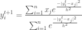
An alternate way to speed up convergence is to alter the data points
during the course of Mean Shift. Again using a Gaussian kernel as
an example,

1. $y_{i}^{0}=x_{i}$
2. $y_{i}^{t+1}=\frac{\sum_{i=1}^{n}x_{j}e^{\frac{-|y_{i}^{t}-x_{j}|^{2}}{h^{2}}}}{\sum_{i=1}^{n}e^{\frac{-|y_{i}^{t}-x_{j}|^{2}}{h^{2}}}}$
3. $x_{i}=y_{i}^{t+1}$

Other Issues

1. Even though mean shift is a non parametric algorithm , it does require the bandwidth parameter h to be tuned. We can use kNN to find out the bandwidth. The choice of bandwidth in influences convergence rate and the number of clusters.
2. Choice of bandwidth parameter h is critical. A large h might result in incorrect
clustering and might merge distinct clusters. A very small h might result in too many clusters.

3. When using kNN to determining h, the choice of k influences the value of h. For good results, k has to increase when the dimension of the data increases.
4. Mean shift might not work well in higher dimensions. In higher dimensions , the number of local maxima is pretty high and it might converge to a local optima soon.
5. Epanechnikov kernel has a clear cutoff and is optimal in bias-variance tradeoff.

Applications of Mean Shift

Mean shift is a versatile algorithm that has found a lot of practical applications – especially in the computer vision field. In the computer vision, the dimensions are usually low (e.g. the color profile of the image). Hence mean shift is used to perform lot of common tasks in vision.

Clustering

The most important application is using Mean Shift for clustering. The fact that Mean Shift does not make assumptions about the number of clusters or the shape of the cluster makes it ideal for handling clusters of arbitrary shape and number.

Although, Mean Shift is primarily a mode finding algorithm , we can find clusters using it. The stationary points obtained via gradient ascent represent the modes of the density function. All points associated with the same stationary point belong to the same cluster.

An alternate way is to use the concept of Basin of Attraction. Informally, the set of points that converge to the same mode forms the basin of attraction for that mode. All the points in the same basin of attraction are associated with the same cluster. The number of clusters is obtained by the number of modes.

Computer Vision Applications

Mean Shift is used in multiple tasks in Computer Vision like segmentation, tracking, discontinuity preserving smoothing etc. For more details see [2],[8].

Comparison with K-Means

Note : I have discussed K-Means at K-Means Clustering Algorithm. You can use it to brush it up if you want.

K-Means is one of most popular clustering algorithms. It is simple,fast and efficient. We can compare Mean Shift with K-Means on number of parameters.

One of the most important difference is that K-means makes two broad assumptions – the number of clusters is already known and the clusters are shaped spherically (or elliptically). Mean shift , being a non parametric algorithm, does not assume anything about number of clusters. The number of modes give the number of clusters. Also, since it is based on density estimation, it can handle arbitrarily shaped clusters.

K-means is very sensitive to initializations. A wrong initialization can delay convergence or some times even result in wrong clusters. Mean shift is fairly robust to initializations. Typically, mean shift is run for each point or some times points are selected uniformly from the feature space [2] . Similarly, K-means is sensitive to outliers but Mean Shift is not very sensitive.

K-means is fast and has a time complexity $O(knT)$ where k is the number of clusters, n is the number of points and T is the number of iterations. Classic mean shift is computationally expensive with a time complexity $O(Tn^{2})$ .

Mean shift is sensitive to the selection of bandwidth, $h$ . A small $h$ can slow down the convergence. A large $h$ can speed up convergence but might merge two modes. But still, there are many techniques to determine $h$ reasonably well.

Update [30 Apr 2010] : I did not expect this reasonably technical post to become very popular, yet it did ! Some of the people who read it asked for a sample source code. I did write one in Matlab which randomly generates some points according to several gaussian distribution and the clusters using Mean Shift . It implements both the basic algorithm and also the adaptive algorithm. You can download my Mean Shift code here. Comments are as always welcome !

References

1. Fukunaga and Hostetler, "The Estimation of the Gradient of a Density Function, with Applications in Pattern Recognition", IEEE Transactions on Information Theory vol 21 , pp 32-40 ,1975
2. Dorin Comaniciu and Peter Meer, Mean Shift : A Robust approach towards feature space analysis, IEEE Transactions on Pattern Analysis and Machine Intelligence vol 24 No 5 May 2002.
3. Yizong Cheng , Mean Shift, Mode Seeking, and Clustering, IEEE Transactions on Pattern Analysis and Machine Intelligence vol 17 No 8 Aug 1995.
4. Mean Shift Clustering by Konstantinos G. Derpanis
5. Chris Ding Lectures CSE 6339 Spring 2010.
6. Dijun Luo’s presentation slides.
7. cs.nyu.edu/~fergus/teaching/vision/12_segmentation.ppt

8. Dorin Comaniciu, Visvanathan Ramesh and Peter Meer, Kernel-Based Object Tracking, IEEE Transactions on Pattern Analysis and Machine Intelligence vol 25 No 5 May 2003.
9. Dorin Comaniciu, Visvanathan Ramesh and Peter Meer, The Variable Bandwidth Mean Shift and Data-Driven Scale Selection, ICCV 2001.