linear algebra | God, Your Book Is Great !!

Posts Tagged ‘linear algebra’

Introduction to PCA – Part 1

Posted in Data Mining, tagged basis, Data Mining, latex, linear algebra, machine learning, pca, stanford on February 4, 2010| 10 Comments »

This series of posts discusses some basic ideas in data mining . For all posts in the series see here.

I got lot of useful feedback on my post on K-means. Most common were to discuss the basic intuition in more detail and to include more figures to clarify the ideas . Thanks people for those comments !

Topic and Organization

In this post , I will discuss about Principal Component Analysis aka PCA , a very popular dimensionality reduction technique. It has an amazing variety of applications in statistics, data mining, machine learning, image processing etc

PCA is a huge topic to cover in a single post. So I plan to write it as a trilogy – First post will talk about PCA in lower dimensions with emphasis on geometric intuition and application to compression. Second post will extend it to arbitrary dimensions and discuss about basic dimensionality reduction , and the two common algorithms for calculating PCA. Third post will discuss Eigenfaces , which is probably one of the coolest application of PCA where we use it for face recognition.

Motivation for PCA

Before discussing PCA per se, let us discuss the reasons why PCA is one of the most important technique in data mining / machine learning. In this post I will primarily discuss with respect to compression. In the next post, we will discuss the more general idea of dimensionality reduction.

Let us assume that we have some arbitrary process that generates (x,y) points in 2 dimensional space . We do not know the behavior/internals of the process but we suspect that there is some inherent relation between x and y. There can be many reasons for trying to know the internal behavior. For eg if we know the relation between x and y, then we need to store only x and the transformation function. For eg if we had 1000 points in 2 dimensions , then we need 2000 words to store them (assuming each number takes word to store ,which is 4 bytes) . But if we knew the relation between x and y, we only need to store 1000 numbers (ie only x) which will occupy 1000 words as we can recalculate y from x using the transformation function. We get a 50% compression !

Let us take an example. Assume that our unknown process, generated some points which when plotted , we get the following graph.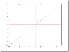

The red lines are the x-y axes and the green crosses are the points generated by the process. The relation between x and y is obvious to us now. The internal logic is $y=x$ . Now if we just store x, then we know how to get y. Some other examples of possible functions are $y=1.8x + 32$ (Celsius to Fahrenheits) or $y=1.6x$ ( miles to kilometers) . These two examples are slightly not very obvious but still we can see that x and y are related by some transformation function. PCA works best when this transformation function is linear. $y=x, y=1.6x, y=1.8c+32 , y=ax+b$ are all linear but $y=x^2$ is not.

Let us discuss the $y=x$ example in slightly more detail. In this simple example, we were able to easily identify the transformation function as the data was in 2 dimensions. In 2 dimensions, the only valid linear transformation is that of a line. But in higher dimensions it will be a (hyper)plane and hence finding the exact linear transformation might be hard to do it just by eyeballing the data. In fact, even visualizing the data in higher dimensions is a big problem. Hence we need a more algorithmic way to find the relation.

Short Detour To Linear Algebra : Vector Spaces and Basis

Basis is one of the fundamental ideas in Linear Algebra. I will give a short discussion of basis here – for more details consult some good book on Linear Algebra or some video lectures on it. For more details on learning it see my post on Linear Algebra .

Before discussing basis, let us talk about Vector Spaces. Intuitively, a vector space is a collection of vectors . It has the additional property that if you take any two vectors in it and add them, the result is also in the original collection. Similarly, if you multiply any vector by a scalar , the result is also in the original collection. So we can say that vector space is a collection of vectors that are "closed" under vector addition and scalar multiplication. A subspace is a similar idea. A subspace is subset of vectors in the original vector space but also have the behavior of a vector space. ie being closed under vector operations.

If the above paragraph sounded very abstract , it isn’t. You can consider the set of all real values vectors representing points in 2 dimensions as vector space. It is represented as $\mathbb R^2$ . If you take any two vectors and add them the result is still in $\mathbb R^2$ . Same goes for scaling.

Now that we have discussed vector spaces, let us talk about Basis. Basis is again a set of vectors. We say that B is a Basis for a Vector Space V , if all the vectors in vector space V can be expressed as a linear combination of the vectors in the basis,B . So the vectors in the basis can express every vector in the vector space as a linear combination of themselves but no vector in a basis can be expressed as linear combination of other vectors in a basis. Wikipedia concisely states this fact – Basis is a "linearly independent spanning set."

The idea of Basis might sound confusing, but an example might clear it. Let us consider all the real valued 2-dimensional points represented by $\mathbb R^2$ . The simplest basis (aka standard basis ) for $\mathbb R^2$ that corresponds to the x-y axes are

$e_1=\left[ \begin{array}{c} 1 \\ 0 \end{array} \right] , e_2=\left[ \begin{array}{c} 0 \\ 1 \end{array} \right]$

We can notice several things in this basis.
a) All the vectors in $\mathbb R^2$ can be represented as a linear combination of $e_1$ and $e_2$ .

$\left[ \begin{array}{c} a \\ b \end{array} \right] = a \times \left[ \begin{array}{c} 1 \\ 0 \end{array} \right] + b \times \left[ \begin{array}{c} 0 \\ 1 \end{array} \right]$

b) The vectors $e_1$ and $e_2$ are the columns of the identity matrix. Also the two vectors are orthogonal. (ie the vectors are perpendicular to each other)
c) More interestingly, the two vectors $e_1$ and $e_2$ are also orthonormal (orthogonal vectors with unit length)
d) We can also notice that this basis corresponds to the standard x-y axes.

An important thing to note is that a vector space might have more than one basis. There are common techniques like Gram-Schmidt to generate Orthogonal sets of vectors. For eg , other valid basis for $\mathbb R^2$ are :

$\left( \left[ \begin{array}{c} 1 \\ 1 \end{array} \right], \left[ \begin{array}{c} 1 \\ -1 \end{array} \right] \right) , \left( \left[ \begin{array}{c} 1 \\ 1 \end{array} \right], \left[ \begin{array}{c} -1 \\ 2 \end{array} \right] \right)$

Change Of Basis

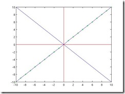
So why did we discuss basis so much ? The reason is that PCA can be considered as a process of finding a new basis which is a linear combination of the original basis such that the inherent structure of points becomes more clear. Most of the time the standard basis (which is the x-y axes) makes a lousy basis. Again, let us see a picture to clarify this idea.

This image is very similar to the previous image. As before, the red lines are the x-y axes and the green crosses are the points. But what are the blue lines ? They are two axes which are perpendicular to each other but have the nice property that they bring out the internal structure more clearly. In other words, they are the new basis. Let us refer them as $u_1$ and $u_2$ .

How is this new basis related to the original basis ? We get the new basis by rotating the original basis by 45 degrees. Remember, rotation, stretching and shrinking of the constituent vectors are all valid linear transformations.

Why is this new basis better than the old one ? Because , in this new basis the original point become (1,0), (2,0) and so on. So we only need one number to represent a point instead of the two in the original basis. We can also think that we have projected points in 2-dimensions to 1-dimension and have got the benefits of compression ! But we know that we can still get all the points back if needed.

A Dose of Real World

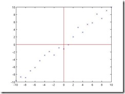
So far we have been living in the ideal world where the sensors gave us perfect data. But in real world , the sensors usually give the data with some noise. So let us take a look at the plot where a gaussian noise is added to the points.

So whatever we discussed above still holds but with slight modifications. Since the data was in 2 dimensions, to get a compression we need to project the points to 1 dimension. So we have to choose to project the points onto one of the axes (basis). How do we select the which axis to project on ? Since the points have noise in them , we need to project the points on to the axis which minimizes the projection error. Let us consider both the cases :

[Image Credit : The following 3 images are obtained from Stanford Prof Andrew Ng‘s Machine Learning course : Lecture notes on PCA ]

Case 1: Here we project on the first vector(axis) $u_1$ . The image with the projection error is here.

Case 2: Here we project on the first vector(axis) $u_2$ . The image with the projection error is here.

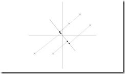
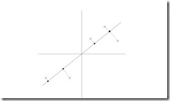
Which projection did you prefer ? I am sure you would have preferred the first projection intuitively. Algorithmically too that is the correct answer. The projection onto vector $u_1$ had lesser projection error than the projection onto vector $u_2$ . In short, PCA selects a basis which is a linear combination of the original basis which also minimizes the projection error. How it does that , we will discuss in the next post.

Alternate View Of PCA

So far we have discussed PCA in terms of change of basis. There is an alternate way of looking at it . This way is slightly less intuitive but is very useful when you want to prove the optimality of PCA or derive formulas for PCA. The new idea is to look at the variance.

Let us take a look at the points again.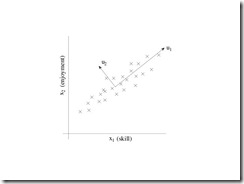

We have to select one of the axis onto which we want to project the points. Which axis should you select ? From the image , vector $u_1$ is in the direction of higher variance than vector $u_2$ . Hence we need to select projection over $u_1$ because that projection tries to maintain more information about the original points than the projection onto $u_2$ . Please look at the images of the actual projection onto $u_1$ and $u_2$ given above. Projection on $u_2$ is bad as some points in the original data might be projected onto a same point in the new axis.

An alternate reasoning is that the original points will be along the direction of highest variance and the noise will be along the direction of the lesser variance. This is because, noise by definition is usually much smaller compared to original data points. Since $u_1$ lies along the direction of highest variance it must lie on the best fit line . $u_2$ being smaller gives the direction of the noise. ( What happens if the noise is too high ? PCA will still work but with very high projection error )

There is a formal proof that shows that minimizing the projection error and maximizing the variance are equivalent. We will skip the proof here.

Summary

The important points in this post are the following :
1. The standard basis is usually a bad one to store data.
2. PCA tries to find a new basis such that the projection error is minimized.
3. Alternate way to look at PCA is that it finds a vector to project which is in the direction of the highest variance.

Read Full Post »

Impressions On MIT OCW Linear Algebra Course

Posted in Data Mining, math, tagged Data Mining, linear algebra, machine learning, mit, ocw on January 30, 2010| 10 Comments »

Linear Algebra is one of the coolest and most useful math courses you can take. Basically , it deals with vectors , matrices all the cool stuff you can do with them. Unfortunately, I did not really have a dedicated course on Linear Algebra in my undergrad. From what I hear , most of the CS people I meet (from India) also don’t have this course in their undergrad. Sure we have had some of the topics (like vectors, basic matrices, determinants, Eigenvalues) split across in multiple courses or in our high school ; but not a single,unified course on it.

Linear algebra is useful on its own but it becomes indispensable when your area of interest is AI , Data Mining or Machine Learning. When I took a machine learning course , I spent most of the time learning things in Linear Algebra, adv Calculus or Linear Optimization. In hindsight , machine learning would have been an easy course if I had previously taken courses on Linear Algebra or Linear Optimization.

As a concrete example, I had a hard time understanding the proof of optimality of PCA or the equivalence of different techniques for calculating PCA (eg Eigen space decomposition or SVD etc) . But once I learnt all about basis, dimension , ,Eigen space and Eigen space decomposition, QR decomposition,SVD etc (which are btw taught in any intro course of Linear Algebra) the whole PCA concept looked really really simple and the proofs looked like straight forward algebraic derivations. Oh well, the benefits of hindsight 🙂

Ok, enough on my rant on lack of Linear Algebra in undergrad. After I struggled mightily in my machine learning course, I decided that I had to master Linear Algebra before taking any more advanced courses. I spent the entire winter holidays learning Linear Algebra as I was taking an advanced data mining course this spring. So this blog post is a discussion of my experience.

Video Resources

Arguably the best resource to learn Linear Algebra is MIT’s OCW course taught by Professor Gilbert Strang . This course are is one the most popular OCW course and so far had more than 1 Million visits . I also searched for alternate courses, but this course wins hands down both for its excellent teaching style and its depth.

The course website is here. It contains around 35 video lectures on various topics. The lecture are available for download both from ITunes and from Internet Archive. If you prefer YouTube, then the playlist for this course is here.

Books

The recommended book for this course is Introduction to Linear Algebra. 4th ed. by Gilbert Strang. I found the book to be quite costly , even used books for old versions ! I don’t mind buying expensive books (I shell out a lot of money for data mining books , but a rant on it later ) but since I was interested in Linear Algebra primarily to help me master data mining, I preferred the equivalent book Linear Algebra and Its Applications , also by Gilbert Strang. This book had a very similar content to the recommended book but I felt was more fast paced which suited me fine. Also I was able to get an old copy from Amazon for 10 bucks. Sweet ! My only complaint of the book is that the examples and exercises felt a bit disconnected (or should I say, I wasn’t clear of the motivation ? ) from the topics.

If you don’t want to purchase these expensive books , then there is an EXCELLENT free e-book by Professor Jim Hefferon .The book’s website is here , from where you can download the e-book. I have to say, this book really blew me away. It was really intuitive, has excellent (mostly plausible) examples, was slightly more theoretical than Strang’s book with more proofs. It also had a very helpful solution manual , and a LaTeX version of the book. Too good to be true 🙂 I felt this book had a much limited set of topics than Strang’s course/book, (hence this a truly intro book) , but whatever topic it took, it gave it a thorough treatment. Another thing I liked in the book are the exercises – Most of them were excellent. And having a solution manual helped clarify a lot of things given that I was doing essentially a self-study. Thanks Jim !

Impressions on the Lectures

I felt, overall, the lectures were excellent. They were short (40-50 minutes). So my usual daily schedule was to listen to a lecture, and read the relevant sections in the book , solve the exercises for which the answers are available at the end of book. All these steps took at most 2-3 hours a day. I was also taking notes in LaTeX using Lyx. I have talked about using Lyx previously in this blog post.

I really liked Strang’s teaching style. He often emphasizes intuition , especially geometric intuition rather than proofs. I felt that is how intro courses must be structured. Proofs are important but not before I have a solid understanding of the topics. But I also have to say that the lectures were varying in quality. Some of the lectures were exceptional while some were not so enlightening. But on the whole, I was really glad that he has made the lectures available online. It has certainly helped me learn Linear Algebra.

Topics

If possible see all the lectures as almost all of them cover important topics. I did and have to say all of them were excellent and useful. But if you are mostly interested in applied Linear Algebra and planning to use it in Data Mining/ Machine learning, then my suggestion will be Lectures 1-11 , 14-22,25,27-29,33. If you are interested watch lectures 30,31 too. Again a better way to learn is to take notes during lectures and solving at least a few exercises in the book. If you have Matlab or Octave then you can verify answers to some other exercises for which solutions are not given.

Notes

I have taken LaTeX notes for this course but they are a bit scattered and unorganized. Hopefully, I will organize them together and create a single PDF soon. I kind of put it on a lower priority after I noticed that Peteris Krumins’s blog has a partial set of lecture notes for this course. His lecture notes can accessed here . As of now (Jan 30 , 2010) , he has put notes for first 5 lectures although the frequency seems to be a bit slow.

Have fun with Vectors and Matrices !!